Stardust Memories

When I was ten, my dad took a couple of friends and me to see a movie. My friends and I had the choice of watching Rollercoaster, which was about a terrorist attempting to extort money from amusement parks by blowing up sections of rollercoaster track just as the coaster gets to them, or this new science fiction film that had recently opened and was getting good notices. As you've no doubt guessed, we chose poorly, while my dad went to the other film, which was (as you've probably also guessed) Star Wars. Meanwhile, one of my friends threw up on the car ride home.

I saw Star Wars in the theater four times, which to this date remains the last time I ever saw a film multiple times in the theater. Early in the film, right after the text crawl, but before the rebel ship comes on screen, you're treated to a view of a star field. In fact, here it is (click to enlarge):

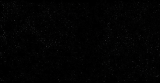
When I saw the film again recently, there was something vaguely unsettling and unnatural about the look of the stars in this scene. For the sake of comparison, here's a real star field, with roughly the same level of detail (again, click to enlarge):

What strikes me now (although I was oblivious to it back in 1977, at least consciously) is how much more regular the star field is in the Star Wars frame than it is in the real photograph. There isn't much variation in the stars in the movie frame, with the top fifty or so being about the same brightness; in contrast (no pun intended), there are many more dim stars in the real photograph, and they fade out gradually, suggesting that there are plenty of stars that are in the field of view, but just beyond the limits of detectability, in this photograph at least. And there are, in fact. For some reason, that sense of infinity, which isn't in the movie frame, appeals to me greatly.

You can sort of see the reasoning behind this if you imagine for the moment that all stars are of the same intrinsic brightness, and that the only reason that some appear brighter and some appear dimmer is that they're closer or further away. (Sort of the way that most adults are of about the same height, but appear to be different sizes because they're at different distances.) And because there is more space far away than there is close up, there are more stars that are far away and therefore dim than there are stars that are close up and therefore bright.

Now, as it happens, stars do vary in actual brightness—sometimes dramatically—but the basic explanation still holds, and is supported by actual counts of bright stars versus dim stars. And I think that through long association with the night sky, we gain an appreciation for that kind of aesthetic. Once upon a time, every human on the planet with reasonably good vision had that association. Nowadays, it's less common. But the potential is still there within each of us, and in my case, it expressed itself in, among other things, my preference for the real star image rather than the Star Wars movie frame.

And this set me to wondering whether a sense for this kind of aesthetic could be mechanized in any way. In a very naïve way, it surely could. The way that the star counts vary by brightness follow a fairly well-understood formula, and a star field could easily be scanned for how well it matches that formula. But I think it's a common feeling that that would fall well short of a genuine sense of aesthetics. There would have to be a larger framework for that kind of aesthetic sense.

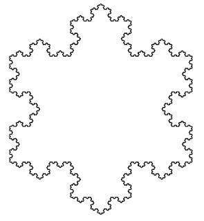
Could such a framework lie in fractals? Fractals are, generally speaking, patterns that are self-similar; that is, the appearance of the whole at a large scale is repeated in small parts of the pattern at smaller scales. Examples of fractals range from prosaic snowflake patterns:

to the sublime Mandelbrot set:

Fractals have been used to describe natural patterns as varied as the sound of wind through trees and the coastline of Great Britain. And they can be used to describe the appearance of star fields as well. A star field looks quite the same if you zoom in and increase the brightness. The details are different, so in that sense it is not quite like the snowflake fractal or even the Mandelbrot set. But statistically, the close-up shot and the wide-angle shot are essentially identical.

I cannot say exactly what it is about the "fractality" of these patterns that is appealing. And it does seem as though a certain sense of variation (absent in the snowflake, present to an extent in the Mandelbrot set, and rampant in real star fields) is vital to maintaining visual interest. But I can't escape the notion that self-similarity is something that people generally find captivating and inviting, once they recognize it, and is a large part of why looking up at the night sky is such a natural thing to do.

Seventh Night

Last night was Seventh Night (七夕), the seventh night of the seventh month in the lunisolar calendar followed traditionally by the Chinese. Because the Chinese calendar usually starts with the second new moon after the winter solstice, Seventh Night usually falls sometime in August in the western calendar.

Seventh Night is associated in Chinese tradition with the story of the Cowherd and the Weaver Girl. In one common telling of the story, a young cowherd by the name of Niulang (牛郎) came across a fairy girl bathing in a lake—a girl named Zhinü (織女). Fascinated by her beauty, and emboldened by his companion, an ox, he stole her clothes and waited by the side of the lake. When she came out looking for her clothes, Niulang swept her up and took her back home. In time, they were happily married with two children. But when the Goddess of Heaven found out that a fairy girl had married a mere mortal, she grew furious and sent Zhinü into the sky, where she became the bright star Vega, in the constellation of Lyra the Lyre. (Watercolor by Robin Street-Morris, 2007.)

When Niulang discovered that his wife had disappeared, he searched high and low for her, but was unable to find her. Eventually, the ox told Niulang that if he killed him and wore his hide, he would be able to ascend the heavens to find Zhinü. Niulang did as the ox suggested, and took his two children with him to find his wife, becoming as he did the star Altair. Find her he did, but the Goddess of Heaven, angered once more by Niulang's impertinence, drew a river of stars—the Milky Way—forever separating Niulang (the star Altair) from Zhinü. Their two children became Tarazed and Alshain, the two dimmer (but still bright) stars that flank Altair in the constellation of Aquila the Eagle. But apparently the Goddess of Heaven was not entirely heartless, for once a year, on the seventh night of the seventh month, she sends a bridge of magpies (鵲橋) to connect the two lovers, for just one evening. And so Seventh Night is associated with romance (and also, interestingly, with domestic skills).

The celestial setting for the entire tale can be found in the Summer Triangle, which is bounded by three stars: Altair, Vega, and Deneb (in the constellation of Cygnus the Swan, also known as the Northern Cross). The Summer Triangle can be found in the night sky throughout summer and autumn; at this time of year, it passes nearly overhead at about ten in the evening. (Photograph by Bill Rogers of the Sa-sa-na Loft Astronomical Society, 2009; click to enlarge.)

How Random is Random?

We all think that we know when something is random. But how random is random?

Part of the aim of mathematics is to unify concepts. It's what makes mathematics more than just a collection of ways to figure things out. As a side effect, though, mathematics definitions tend to be a bit counterintuitive. For example, I think we all know what the difference between a rectangle and a square is: A square has all four sides of equal length, and a rectangle doesn't.

Except that a mathematician says that squares are rectangles, because to a mathematician, it's inefficient and non-unifying to say that a rectangle is a four-sided figure with four right angles, except when all four sides have the same length. It makes more sense, from a mathematical perspective, to make squares a special case of rectangles.

So hopefully it won't come as too much of a surprise if I say that a completely deterministic process, such as flipping a coin that always comes up heads, is still considered a random process to mathematicians who study that sort of thing. So is a coin that comes up heads 90 percent of the time. Or 70 percent. Or—and maybe this is the surprise, now—50 percent. The cheat coin is simply a special case of a random process. To a mathematician, none of these processes is "more random" than the others. They just have different parameters.

What we think of as randomness, mathematicians call entropy. This is related to, but not the same thing as, the thermodynamic entropy that governs the direction of chemical reactions and is supposed to characterize the eventual fate of the universe. (Another post, another time, perhaps.) It turns out that this "information-theoretic" notion of entropy corresponds pretty well to what the rest of us call randomness. For those of you who are even the slightest bit curious, the definition of entropy for a flipped coin is

S = - ( p_H lg p_H + p_T lg p_T )

where p_H and p_T are the probabilities for heads and tails, respectively, and lg is logarithm to the base 2. For a 50-50 coin, the entropy is S = 1; for a completely deterministic coin (a two-headed one, for instance), the entropy is S = 0. For something in between—say, one that comes up heads 70 percent of the time—the entropy is something intermediate: in this case, S = 0.88 approximately.

So, all right, how entropic is a real coin? The answer is that it's probably less entropic—less random, that is—than you think it is, especially if you spin it. A paper by researchers from Stanford University and UC Santa Cruz (via Bruce Schneier, in turn via Coding the Wheel) has seven basic conclusions about coin flips:

1. If the coin is tossed and caught, it has about a 51 percent chance of landing on the same face it was launched. (If it starts out as heads, for instance, there's a 51 percent chance it will end as heads.)
2. If the coin is spun, rather than tossed, it can have a much larger than 50 percent chance of ending with the heavier side down. Spun coins can exhibit huge bias (some spun coins will fall tails up 80 percent of the time).
3. If the coin is tossed and allowed to clatter to the floor, this probably adds randomness.
4. If the coin is tossed and allowed to clatter to the floor where it spins, as will sometimes happen, the above spinning bias probably comes into play.
   
5. A coin will land on its edge around 1 in 6000 throws.
6. The same initial coin-flipping conditions produce the same coin flip result. That is, there's a certain amount of determinism to the coin flip.
   
7. A more robust coin toss (more revolutions) decreases the bias.

Somewhat along the same lines, Ian Stewart, who for a while wrote a column on recreational mathematics for Scientific American, mentioned a study in one of his columns by an amateur mathematician (and professional journalist) named Robert Matthews. Matthews had watched a program in which the producers had asked people to toss buttered toast into the air, in a test of Murphy's Law as it applies to buttered toast. Somewhat to their surprise, the toast landed buttered side up about as often as it landed buttered side down.

Matthews decided that was not quite kosher. People, he thought, don't usually toss buttered toast into the air; they accidentally slide it off the plate or table. That ought to be taken into account when analyzing Murphy's Law of Buttered Toast. And when he did take it into account, he found something rather unusual. A process that you might have thought was fairly entropic turned out to be almost wholly deterministic, given some not-so-unusual assumptions about how fast the toast slides off the table. Unless you flick the toast off the table with significant speed, the buttered side lands face down almost all of the time. And it has nothing to do with the butter making that side heavier; it's that the rotation put on the toast as it creeps off the table is just enough to give it a half spin. Since the toast starts out buttered side up (one presumes), it ends up buttered side down. Stewart recommends that if you do see the toast beginning to slide off the table, and you can't catch it, to give it that fast flick, so that it isn't able to make a half flip, and lands buttered side up. You won't save the toast, unless you keep your floor fastidiously clean, but you might save yourself the mess of cleaning up the butter.

On the other hand, maybe there's another solution.

Lines for Fries (and Fry's)

Thoughts about (and while) waiting in line at the neighborhood McD's. Mmm...fries.

The Most Evil Being mocked the last queueing theory post, but he actually read the whole thing to mock it. Apparently, so did Squishy. I approve, of course. But Squishy noticed, with some temerity, that I had tagged that post with "queueing theory," indicating a potential for future posts about same. Well, the future is now. That post dealt with queueing theory itself as little as I could manage, which, OK, is still quite a bit, I guess. Fair warning: There's a bit more of it in this one.

If you were so foolhardy as to look in a queueing theory textbook, you'd probably see a representation of a queue as something like this:

The thing at the left is the queue, or waiting line; the colored blocks inside the queue represent customers; and the circle at the right is the server. Nowadays, in the computer world, we think of servers as big honking machines, but in general, it could be anything that provides a service. Say, an order taker at a fast food restaurant.

That diagram up there represents only one potential way to hook customers up with servers: a single queue with a single server. Lots of places, like McDonald's, or the supermarket, or the bank, have multiple servers available at a given time. How do they connect their customers to their servers? Here are two diagrams representing two options, without any explanation. Before reading on, see if you can figure out what queueing systems they represent, and how the lines you wait in everyday are arranged.

System (a), on the left, represents a queueing system in which each server (e.g., checkout clerk, bank teller, etc.) has his or her own line. System (b), on the right, represents a system in which all the servers together share a single line. Where I live, in Los Angeles, McDonald's and the supermarket use (a), and the bank and some other fast food places use (b). Your mileage may vary, of course.

OK, that wasn't too hard, probably. Now think about this one: All other things remaining equal, which system is better? And by better, I mean that it improves the time that you have to wait, on average, before getting service. We'll assume, to make things easier, that once you enter a queue or line, you stay in it; you don't give up, and you don't defect to another line. We'll also assume, furthermore, that all the servers are equally fast (or slow, depending on your point of view). Would you prefer to wait in (a), or (b)?

Before I answer that, let me first define some terms. All queueing systems have what's called an arrival rate, which is the rate, on average, at which new customers enter the queueing system. All servers have a service rate, which is the rate, on average, at which they can serve customers, assuming they have any customers to serve. One of the things I mentioned in that last queueing theory post was that a system is stable (that is, it doesn't jam up) if the arrival rate doesn't exceed the service rate. With me so far?

All right, one last term: The utilization of a server, or a group of servers, is the arrival rate divided by the service rate. So, pretty obviously, if the utilization of a server or servers is less than one, it's stable, and if it's greater than one, it's unstable—the line or lines get longer and longer. Somewhat less obviously, the utilization of a server is also the fraction of time that it spends actually serving customers, rather than sitting idle (which is why it's called the utilization in the first place).

Suppose Store A is using queueing system (a). It's got, let's say, six servers, each capable of serving one customer a minute. Customers come into the store at a rate of three customers a minute. Since each server gets one-sixth of all the customers, on average, each server's customer arrival rate is half a customer a minute, and each server's utilization is 1/2 divided by 1, or 1/2.

Store B, on the other hand, is using queueing system (b). It also has six servers, each of which also serve at one customer a minute. Because they all get fed from the same line, it's convenient to think of them as together serving customers at a rate of six customers per minute. If the arrival rate to Store B is the same, three customers per minute, then the utilization of the six servers, combined, is 3 divided by 6, or again, 1/2. So far, it seems like the two systems are pretty equivalent.

However, Store A has a problem that Store B doesn't. Consider the situation diagrammed below:

Five of the servers are busy, and they even have customers waiting in line behind them. The sixth server, however, is entirely idle, but because we've assumed that customers don't switch lines, it has nobody to serve. (Lest you think this is entirely unrealistic, I see it all the time at the supermarket, possibly because the idle server is a few counters away from the busy ones.) This is bound to happen from time to time, since the utilization is less than one. Servers are going to be idle every now and then, and if that happens when some other customers are waiting to be served, Store A is going to be inefficient at those times.

Note that this never happens to Store B. Certainly, servers are going to be idle from time to time, and customers are going to have to wait from time to time. But they never both happen at the same time. Any time a server comes idle, if there's any customer waiting for service, it can go straight to that server. As a result, Store B, and queueing system (b), is better for the customers: They wait for a shorter time, on average, than customers at Store A.

What's more, queueing system (b) is fairer, in the sense that customers that arrive first are served first. That doesn't always happen with queueing system (a). In the situation depicted above, if a customer now arrives to that sixth, idle server, it gets served immediately, without having to wait, even though customers that arrived previously to other lines are still waiting. So (b) is doubly better than (a).

In light of this, it shouldn't come as any surprise that Fry's Electronics, essentially the store for übergeeks, uses system (b) in every one of its stores I've been in. It even takes advantage of the longer single line (as opposed to an array of shorter lines) by snaking it between and amongst a panoply of impulse buys. One could argue that supermarkets can't really take proper advantage of system (b), because people usually have carts, and these take up a lot of room, which would obstruct other supermarket traffic. (I also haven't considered the effect of the 12-items-or-less express lanes.)

But a place like McDonald's has no such excuse. Even if you make the point that people switch lines when there's nobody waiting at a server (because the service counter is not so large), it's still unfair, in that it's not first-come-first-served. And other fast food places are perfectly willing to arrange a single line for all servers.

Coke, Currency, and Contagion

Recently, there was a report, from the American Chemical Society, that about 90 percent of U.S. currency in circulation has detectable traces of cocaine on it. Apparently, the middle currencies—from Lincoln on up through Jackson—are the most susceptible. I guess Washington and Franklin don't rate. Also, not surprisingly, the percentage varies according to the community. Rural areas are less hit by cocaine-laden dollar bills, but in major metropolitan centers, essentially every piece of currency has coke on it. What's more, the percentage appears to be rising. In 1985, a study found that anywhere from a third to a half of bills had cocaine on them; in 1995, the proportion was three in four; and in 1997, it rose to four in five. Now it's nine in ten.

No need to panic, though. First of all, the traces are generally tiny, much smaller than a grain of sand, and not enough to get any kind of buzz from. And secondly, probably much, though apparently not all, of this increase has to do with the improved sensitivity of the cocaine sniffing tools.

The question is, how does cocaine get on all these bills? Certainly not all of the bills get cocaine on them because they were directly around the stuff, either during deals or during use. A small number do, of course, but the vast majority get them through contamination. But is that really plausible? Can so many bills be contaminated so quickly?

Well, let's take a look at that. Suppose that, initially, some small fraction of all the dollar bills have detectable cocaine on them; these are the initial set that get cocaine on them through direct contact with bulk quantities of the drug. Let's call this proportion p. The money isn't discarded, generally; it's put back into circulation (let's not get into how they get put back into circulation). Once that happens, those bills come into contact with other bills, which pick up some proportion of the drug. Apparently, there's an attraction between the drug particles and the green ink used to print U.S. currency.

When I use a bill, and it goes somewhere else, it now comes into contact with, let's say, one new bill. If a contaminated bill comes into contact with another contaminated bill, nothing happens to p, of course; both bills were already contaminated. Same thing holds true if an uncontaminated bill comes into contact with another uncontaminated bill.

But if the bill I had was contaminated and its new companion wasn't, or vice versa, then one new bill gets contaminated. The probability of this happening depends on the current value of p; specifically, it must be proportional to p (1 - p), since we need a contaminated bill and an uncontaminated one. We can put this in terms of a differential equation:

dp / dt = kp (1 - p)

The constant of proportionality k indicates how quickly bills come into contact with one another, and can be eliminated by setting the unit of time equal to the mean time it takes for a bill to be used (and therefore find a new neighbor). I don't have any hard figures, but from my own, non-cocaine-related currency use, it seems to be about a week or so. We can then set k = 1 and solve this equation fairly straightforwardly to yield the formula

p = C e ^t / (1 + C e ^t )

where C is closely related to the initial proportion of contaminated bills. (To be exact, C = q / (1 - q), where q is the initial proportion. Where q is very small, as in most cases, the two are almost exactly the same.) As t increases, C e ^t gets large pretty quickly, and p very quickly approaches 1. If, for instance, q = 0.000001—that is, one bill in a million is contaminated directly by the drug—then it takes a bit more than three months for the fraction of contaminated bills to exceed one-half. But because of the rapid growth of the exponential function, it takes only one more week for the proportion to exceed three-fourths. By the end of the fourth month, the fraction of uncontaminated bills is less than one percent. (Click to enlarge.)

That exceeds even the ACS's report. Why? Well, for one thing, even today's instruments are not perfectly sensitive; there still remain bills with undetectable traces of cocaine, surely. And after a while, there just isn't enough cocaine to go around (for the bills, that is). If, for the sake of argument, we assume that the initial fraction is one in a million, then the ACS's estimate of 90 percent contamination indicates that that first direct contamination can only be split about twenty times before it drops below undetectability.

But a second reason is that bills don't stay in circulation forever. According to the U.S. Treasury, currency stays in circulation, on average, for about 20 months—about 85 to 90 weeks. This makes the dynamical solution to the differential equation a bit more complicated. Let's simplify matters and only look at the equilibrium solution. At equilibrium, the contaminated dollar bills being taken out of circulation each week equal those being contaminated by new contact each week. That is,

p (1 - p) = rp

which yields an equilibrium solution of p = 1 - r, where r is the fraction of bills being taken out of circulation each week (about 1/85 to 1/90). So even with this new influx of bills, if detection tools were perfect, they'd detect traces of cocaine on about 99 percent of bills. Apparently, we still have a few rounds of "alarming" reports about cocaine contamination of currency to look forward to.

OK, here's a less overblown concern. The same model can essentially be used to analyze long-lived infections (such as oral herpes, which infects about 60 to 70 percent of all people worldwide). Such infections are removed from the population only when a person dies. As the above models show, if people were immortal, they'd eventually all be infected with such diseases (and in fairly short order, too). Of course, such diseases couldn't incapacitate their hosts too much, because otherwise they'd fail to be transmitted.

Queueing Theory and You

Some thoughts on traffic—the automobile kind, not the network kind—while there's maintenance work going on in the office across the hall.

So the other day I'm driving into work, and I encounter not one but two traffic jams. Neither, as it turns out, was due to particularly heavy traffic loads. Rubbernecking (a.k.a. looky-looing) was the culprit in both cases. In both cases, the accident/attraction was off to the side of the road but managed to clog up the roads all the same.

I think it's generally underappreciated how much rubbernecking contributes to traffic jams. No one disputes that the accident itself can precipitate the jam. But a moment's satisfaction of curiosity? On the surface, it seems innocuous, right? As one of the drivers stuck in the jam yourself, you've already spent 10, 15, 25 minutes waiting behind this long line of cars—what could it possibly hurt to glance over for a second or two? But it's precisely that kind of glance that keeps the jam going. The reason for this lies in queueing theory, the study of waiting in lines, and comes about from the interplay between the level of traffic applied to a road, and the carrying capacity of the road.

Roads, like any other conduit, have a certain capacity, which is related to the size of the road but is also determined in large part by driving habits. You're taught, when you're driving, to leave at least three seconds of space between you and the car in front of you—more if it's dark or rainy or whatever. In the Los Angeles area, where I live, it's essentially impossible to do this; if you try, someone will invariably slide into the space, cutting yours down to a second or two, after which your options are to either to stay up close, or to back off until you're three seconds behind the new car, in which case the process repeats.

But actually the exact time is not all that important; what's important is that there is a characteristic following time, which determines the carrying capacity of the road. If the following time is two seconds, then the road can carry half a car per second (per lane). Note that this capacity is roughly accurate no matter how fast the traffic is going—whether traffic is flowing at the speed limit or crawling at 15 mph—as long as the following time is roughly the same. Only when traffic slows so much that cars take a significant time to travel their own body length (the following distance isn't head-to-head, but tail-to-head) does this rule break down.

Provided that that doesn't happen (and we'll get to that in a moment), we can now apply the most basic rule of queueing theory: If the amount of traffic going onto the road is more than the road's carrying capacity, traffic will come to a standstill. Hardly earthshattering news. If the amount of traffic is less than the capacity, traffic can flow. It might, however, flow incredibly slowly.

At first flush, this might sound kind of strange. If a road can carry a car every two seconds, and one car comes down the road only every three seconds on average, shouldn't there be enough room for cars to drive smoothly down the road, with quite a bit to spare? The perhaps surprising answer is that there might not be, and the fault lies in that phrase "on average."

If cars all scrupulously observed at least a two-second following time, and entered the road exactly three seconds after the previous car, then in fact, the cars would be able to flow at the speed limit. They would continue to do so even as you increased the rate of cars entering the road, up until the exact moment when that rate exceeded the capacity. At that point, the cars would start backing up and you'd get a traffic jam. And if you've ever been in a large traffic jam, it might seem that that's exactly what happened.

But that isn't in fact what happens. Generally speaking, the capacity of the road is not exceeded for long stretches. It's just very close. So why doesn't traffic flow smoothly, if the traffic load is less than the capacity? There are a few reasons, but the predominant one is that cars do not observe consistent following time, and don't enter the road at a constant rate. In queueing theory, variation kills.

Suppose that the following time is always at least two seconds, but that cars enter the road every three seconds only on average. Sometimes it's less, sometimes it's more. If it's less—let's say it's a second and a half—the new car now has to wait a half a second before it can proceed, because it's trying to maintain a minimum two-second following distance. On the other hand, if it's more, it doesn't have to wait at all. But it also doesn't try to speed up to catch up to the previous car; it's not trying to maintain exactly a two-second following distance, just a minimum of two seconds.

In short, if the time between successive cars is low enough, it slows traffic down, but no amount of time between cars will speed the traffic up. What's more, the closer the traffic rate gets to capacity, the more often a cluster of cars will arrive to slow down traffic, while the gaps between the clusters still fail to speed it up. We can express this effect graphically, by plotting traffic waiting time (a measure of the intensity of the traffic jam) as a function of the traffic rate R.

The exact shape of this graph depends on how following time and the time between cars entering the road vary randomly, but the basic effect is consistent: Instead of the waiting time (the blue curve) being constant at zero until R reaches the road's capacity C, it actually begins ramping up immediately, slowly at first but with increasing intensity until it spikes upward just as it approaches C (the dotted red line). And when you get close enough to C, the waiting time T gets large enough that you notice it as a honest-to-goodness traffic jam.

So what happens when people rubberneck? Yes, it's true, you might have been waiting for a long time, and you're only looking for a second or two. And you're still kind of driving at the time. But you slow down, just for a split second, and increase your following time. Instead of maintaining a minimum two-second following time, you increase it, maybe to two-and-a-half seconds. And if most everybody does this, the capacity of the road is effectively decreased, by 20 percent. It would have the same effect as closing one lane of a five-lane highway.

You might expect this to increase the waiting time T by 20 percent, but actually, what effect this has depends on how high R is compared to C. If it's relatively low—if we're on the left side of the curve—then moving C down by 20 percent, while keeping R the same, doesn't really affect T very much. But if it's already kind of high (and in Los Angeles, at least, it's that high about 24 hours every day), then moving C down by 20 percent can move you catastrophically high up that blue curve, increasing T many-fold and changing a mild nuisance into a dinner-delaying, or even dinner-cancelling, jam.

But that's OK. You just go ahead and look at that upside-down pickup. What could it hurt?

Slashed Back

I'd like to call your attention to our latest scourge: Well-meaning radio announcers who, while reading out URLs in commercials, refer to the ordinary slash (/) as a "backslash." Why they feel compelled to even use the word "backslash," goodness only knows, since most people only ever come into contact with the ordinary slash; the backslash is almost exclusively used by DOS and LaTeX heads.

We now return you to your regularly scheduled rant.